User Guide

A basic workflow of bimato includes loading some 3D image data into a numpy ndarray, calling one of the algorithms provided and storing or plotting the gained data. This tutorial illustrates the a typical workflow to calculate pore-sizes of a Leica LIF image utilizing a third-party python library.

For the sake of clarity, this tutorial analyzes a 2D image. This makes understanding the algorithm and analysis steps a lot easier for the reader. You can find a 3D rendering at the bottom of the page.

Load Data

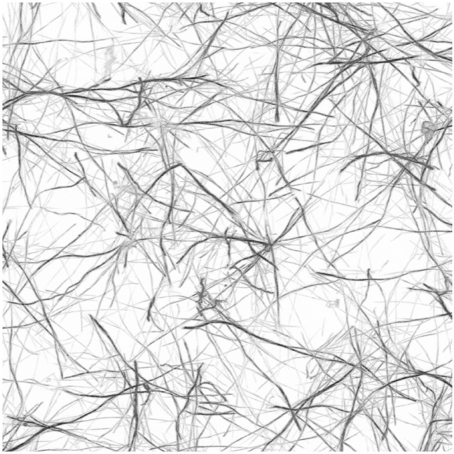
The first step is to load some 3D image data of a biopolymer network as a numpy ndarray. In this tutorial, we will use some LSM image of a fluorescently stained collagen scaffold, recorded using a Leica SP8 LSM. White areas are the fluid phase, black represents stained collagen fibers:

We begin by utilizing the third-party library readlif to conveniently load a single Leica LIF image:

from readlif.reader import LifFile
import bimato

lif_file = LifFile("/path/to/sample.lif")
lif_image = lif_file.get_image(0)

and read a specific 2D image as a numpy ndarray:

data = lif_image.get_frame(z=0, t=0, c=0)

There is a convenience function to load a 3D image under bimato.utils.read_lif_image():

data = bimato.utils.read_lif_image(lif_image)

If the image data has a lot of noise, we can optionally denoise the loaded image using bimato.utils.denoise_image():

data = bimato.utils.denoise_image(data)

Segmentation

We than perform the first fundamental step of image segmentation, where we classify our image into fluid and polymer phase. This is done using bimato’s custom algorithm as published in our article about pore-sizes:

bw = bimato.get_binary(data)

resulting in such a segmentation binary image:

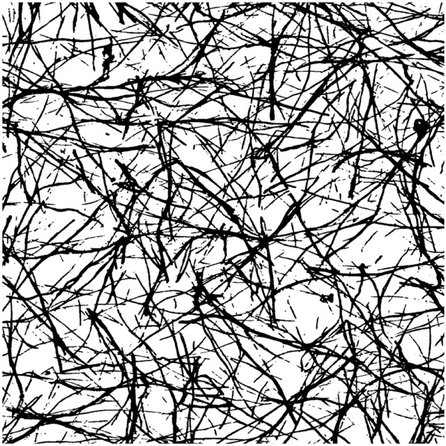
This binary image is the basis for almost all bimato algorithms, such as pore-size, fiber thickness and network structure.

Pore-Size

In this tutorial, we will calculate the pore-size of the collagen scaffold using bimato.get_pore_sizes. It takes a binary image of fluid and polymer phase and the respective image sampling. The parameter sampling needs to be a python dictionary containing the physical pixel size in each x, y and z direction. In this example, we used readlif, which conveniently reads this kind of meta-data for us as an info property of the lif_image.

Note

Keep in mind that bimato.get_pore_sizes expects the physical size in each direction as in “microns per pixel”, not as a scale factor as in “pixel per microns”!

Providing the binary image bw and correct sampling, we receive a pandas.DataFrame:

sampling = {
    'x': 1/lif_image.info["scale"][0],
    'y': 1/lif_image.info["scale"][1],
    'z': 1/lif_image.info["scale"][2]
}

df = bimato.get_pore_sizes(binary=bw, sampling=sampling)

This DataFrame contains every calculated data in several columns. Below is a comprehensive list of all columns and the meaning behind each:

column	data
x [px]	x coordinate in pixel
y [px]	y coordinate in pixel
z [px]	z coordinate in pixel
Diameter [µm]	pore diameter
Residual Degree	number of iterative pore detections, 0 for first step, 1 for second
Size x [px]	total x size of 3D image
Size y [px]	total y size of 3D image
Size z [px]	total z size of 3D image
PhysicalSize x	pixel-micron conversion factor used
PhysicalSize y	pixel-micron conversion factor used
PhysicalSize z	pixel-micron conversion factor used
Number Of Pores	total number of detected pores in sample
Cube Volume [µm³]	physical volume of 3D image
Single Pore Volume [µm³]	volume of detected pore
Real Pore Volume [µm³]	physical volume occupied by detected pores, without overlapping of individual pores
Collagen Volume [µm³]	volume of the polymer phase
Fluid Volume [µm³]	volume of the fluid phase
Single Pore Volume Fraction	space occupied in relation to the sample volume
Real Pore Volume Fraction	space occupied in relation to the sample volume
Collagen Volume Fraction	space occupied in relation to the sample volume
Fluid Volume Fraction	space occupied in relation to the sample volume
Zeta Single Pores	pore diameter scaled with its corresponding column fraction
Zeta Real Pores	pore diameter scaled with its corresponding column fraction
Zeta Collagen	pore diameter scaled with its corresponding column fraction
Zeta Fluid	pore diameter scaled with its corresponding column fraction
Pseudo Pore Diameter [µm]	theoretical pore diameter calculated by assuming that all detected pores would occupy the fluid-phase fully

Each row of the DataFrame contains exactly one found pore. The most interesting value might be Diameter [µm], which is the diameter of the fitted sphere or in other words the “pore” that has been detected. As published in our article about pore-sizes, bimato calculates an exceptionally precise amount of pores with a huge coverage of fluid phase volume:

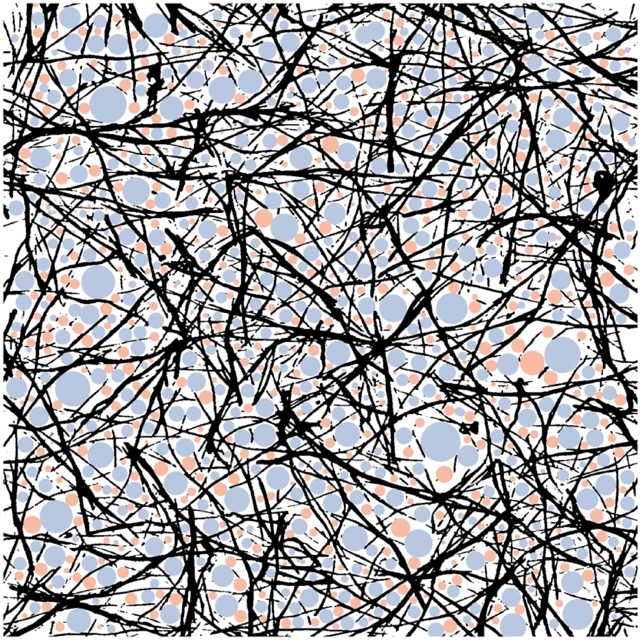
This is illustrated in the image above, where blue pores represent detected pores in the first analysis step, and orange pores represent additional pores detected in a second analysis step, providing a much higher coverage.

Inhomogeneity

In this tutorial, we will calculate the inhomogeneity of the collagen scaffold using bimato.get_pore_sizes and bimato.get_pore_sizes as described in article about inhomogeneity We need the binary image bw (calculated above), correct sampling and define a desired part sie in micron. For example, if our original image is 150 cubic microns, we could split the sample in 30 microns and get a 5x5x5 split. Any arbitrary number is possible and remaining spaces are ignored, for example if we chose a part size of 70 microns, we would end up with a 2x2x2 70 micron parts and remaining 10 micron space.

Note

The part size highly depends on the structure of the biopolymer network and underlying analysis question and can be varified by calculating the inhomogeneity for a range of part sizes.

Providing the binary image bw, correct sampling and the disired part size in micron, we receive a pandas.DataFrame with the same columns as desccribed in bimato.poresize.get_pore_sizes(). However, it is extended by several columns containing the start and end coordinates of each part inside the original data, a unique slice-ID which can be used for example in pandas.DataFrame.groupby(), and several other data columns that are neccessary to calculate the inhomogeneity using bimato.poresize.calc_inhomogeneity(). Subsequently, this data can be used to calculate the inhomogeneity of a particular sample:

frag_df = bimato.get_fragmented_poresizes(binary=bw, sampling=sampling, part_size_micron=30)
inhomogeneity = bimato.calc_inhomogeneity(frag_df)

Exemplary analysis workflow

Usually, we have for example different collagen scaffolds and want to compare structural parameters. For this, we would load several images, calculate their structural parameters and plot them. Below is an exemplary workflow for this:

• load each image in the LIF file

• analyze it

• extract meta-data such as collagen concentration from image name

• concatenate this data to global DataFrame

• plot comparison boxplot

Pore-Size

We load a lif file with multiple samples per collagen concentration and analyze these in a loop:

import pandas as pd
from readlif.reader import LifFile
import seaborn as sns
import bimato

lif_file = LifFile("/path/to/sample.lif")

df_poresize = list()
for lif_image in lif_file.get_iter_image():

    data = bimato.utils.read_lif_image(lif_image)
    bw = bimato.get_binary(data)

    sampling = {
        'x': 1/lif_image.info["scale"][0],
        'y': 1/lif_image.info["scale"][1],
        'z': 1/lif_image.info["scale"][2]
    }

    df_tmp = bimato.get_pore_sizes(binary=bw, sampling=sampling)

    df_tmp['Concentration [g/l]'] = lif_image.name
    df_poresize.append(df_tmp)

df_poresize = pd.concat(df_poresize)

g = sns.catplot(
    data=df_poresize,
    kind='box',
    x='Concentration [g/l]',
    y='Diameter [µm],
)
g.set_ylabels("Pore-size [µm]")

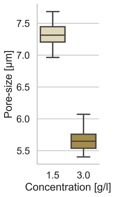
Resulting in the following plot:

Inhomogeneity

We load a lif file with multiple samples per collagen concentration and analyze these in a loop:

import pandas as pd
from readlif.reader import LifFile
import seaborn as sns
import bimato

lif_file = LifFile("/path/to/sample.lif")

df_inhomogeneity = list()
for lif_image in lif_file.get_iter_image():

    data = bimato.utils.read_lif_image(lif_image)
    bw = bimato.get_binary(data)

    sampling = {
        'x': 1/lif_image.info["scale"][0],
        'y': 1/lif_image.info["scale"][1],
        'z': 1/lif_image.info["scale"][2]
    }

    df_tmp = bimato.poresize.get_fragmented_poresizes(binary=bw, sampling=sampling, part_size_micron=30)
    df_tmp['Inhomogeneity'] = bimato.poresize.calc_inhomogeneity(df_tmp)

    df_tmp['Concentration [g/l]'] = lif_image.name
    df_inhomogeneity.append(df_tmp)

df_inhomogeneity = pd.concat(df_inhomogeneity)

g = sns.catplot(
    data=df_poresize,
    kind='box',
    x='Concentration [g/l]',
    y='Inhomogeneity,
)

Resulting in the following plot: